Back Propagation

Backpropagation is an algorithm used by artificial neural network for learning through input data. It is a mechanism in which errors in the network are propagted backwards so that they can be minimized using algorithm like gradient descent. It learns by iteratively processing data set of training tuples, comparing prediction for each tuple with target value. The target value can be either class or numbers. For each training tuple the weights are modified so as to minimize loss function between predicted and actual value. These predictions are made from output layer to hidden layer to input layer so it got its name backpropagation.

Here, we will discuss backpropagation algorithm steps in detail.

Firstly, we have to initialize weights with small random numbers like -0.5 to 0.5 or -1 to 1. They also will have some bias.

Then a input I is passed to network with output as O. Then input of current layer is calculated as:

$$I_{j} = \sum_{i=1}(w_{ij}jO_{i} + θ_{j})$$

Where $w_{ij}$ is weight from unit i in previous layer to unit j. $O_{i}$ is output of unit i from the previous layer. $θ_{j}$ is bias of the unit.

The net input is passed through activation layer to get output as

$$O_{j} = \frac{1}{1 + e^-I_{j}}$$

Similar process is carried to get output in output layer.

Hence, the error is propagated backward by updating weights and biases to reflect error of network prediction. For unit j in the output layer, the error $Err_{j}$ is computed by

$$Err_{j} = O_{j} * (1-O_{j}) * (T_{j} - O_{j})$$

Here $O_{j}$ is actual output of unit j. $T_{j}$ is known target value of given training tuple.

$$To compute error of hidden layer j the weighted sum of units connected to unit j in next layer is considered. The error of a hidden layer unit j is$$

Here, $w_{jk}$ is the weight of connection from unit j to unit k in next higher layer $Err_{k}$ is the error of unit k.

The weight and biases are updated to reflect the propagated errors. Weigths are updated by the following equations where $Δw_{ij}$ is the change in weight $w_{ij}$

$Δw_{ij} = l(Err_{j})O_{i}$ $w_{ij} = w_{ij} + Δw_{ij}$

Here l i learning rate. Backpropagation uses gradient descent technique to search for weight that minimizes cost function of the network.

Bias is updated using following equation.

$Δθ_{j} = l(Err_{j})$ $θ_{j} = θ_{j} + Δθ_{j}$

We can update bias and weight at each iteration or epoch.

When $Δw_{ij}$ in previous epoch are very small or if certain number of epoch is complete the training stops.

Now lets look into a numerical example of backpropagation gradient descent method.

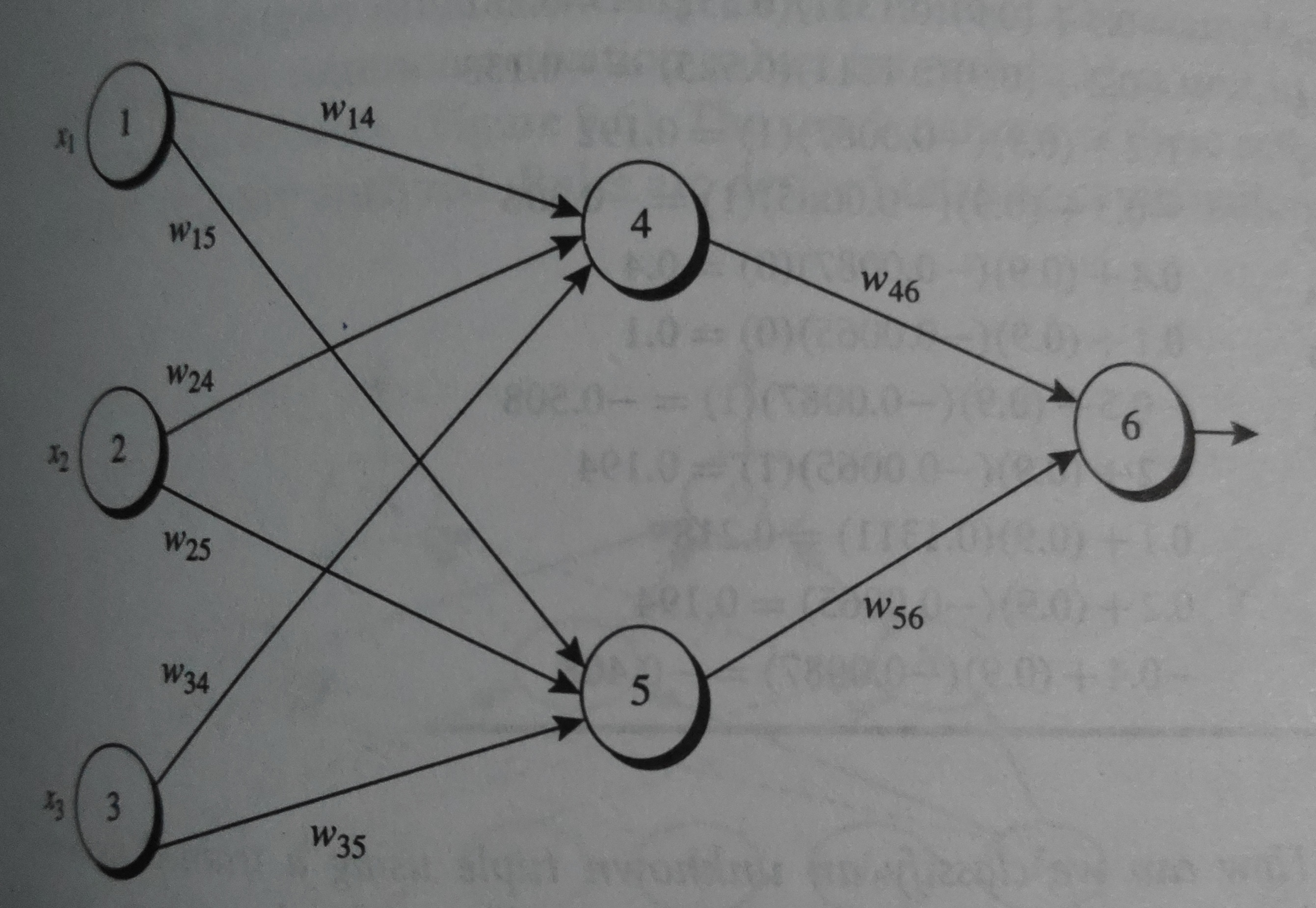
Initial input, weight and bias is given as:

$x_{1}$	$x_{2}$	$x_{3}$	$w_{14}$	$w_{15}$	$w_{24}$	$w_{25}$	$w_{34}$	$w_{35}$	$w_{46}$	$w_{56}$	$θ_{4}$	$θ_{5}$	$θ_{6}$
1	0	1	0.2	- 0.3	0.4	0.1	- 0.5	0.2	- 0.3	- 0.2	- 0.4	0.2	0.1

Net Input and Output is calculated as:

$Unit j$	$Net Input I_{j}$	$Output O_{j}$
4	0.2 + 0 - 0.5 - 0.4 = - 0.7	$/frac{1} {1 + e^0.7} = 0.332$
5	- 0.3 + 0 + 0.2 + 0.2 = 0.1	$/frac{1} {1 + e^-0.1} = 0.525$
6	-0.3 _ -0.332 - 0.2 _ 0.525 + 0.1 = -0.105	$/frac{1} {1 + e^0.105} = 0.474$

Calculation of error at each node as :

$Unit j$	$Err_{j}$
6	0.474 _ (1 - 0.474) _ (1 - 0.474) = 0.1311
5	0.525 _ (1 - 0.525) _ 0.1311 _ ( - 0.2 ) = - 0.0065
7	0.332 _ (1 - 0.332) _ 0.1311 _ ( - 0.3 ) = - 0.0087

Weight and Bias is updated as:

$Weight or Bias$	$New Value$
$w_{46}$	- 0.3 + 0.9 _ 0.1311 _ 0.332 = - 0.261
$w_{56}$	- 0.2 + 0.9 _ 0.1311 _ 0.525 = - 0.138
$w_{14}$	0.2 + 0.9 _ ( - 0.0087 ) _ ( 1 ) = 0.192
$w_{15}$	- 0.3 + 0.9 _ ( - 0.0065 ) (1) = -0.306
$w_{24}$	0.4 + 0.9 _ ( - 0.0087 ) _ 0 = 0.4
$w_{25}$	0.1 + 0.9 * ( - 0.0065 ) _ 0 = 0.1
$w_{34}$	- 0.5 + 0.9 _ (- 0.0087 ) _ 1 = -0.508
$w_{35}$	0.2 + 0.9 * ( - 0.0065 ) _ 1 = 0.194
$θ_{6}$	0.1 + 0.9 _ 0.1311 = 0.218
$θ_{5}$	0.2 + 0.9 * ( - 0.0065 ) = 0.194
$θ_{4}$	- 0.4 + 0.9 _ ( - 0.0087 ) = - 0.408

This same process can be used for network with more hidden layers and neurons.

References:
1.Data Mining: Concepts and Techniques Author: Jiawei Han